HOMER

Based on the protocol for high-throughput sequencing, it is possible to end up sequencing the "same fragments" over and over again.  This happens when the amount of starting material (i.e. IP DNA) is relatively small.  After amplification and cluster generation, several clusters can result from the same single piece of DNA that was found in the initial IP.

In the case of sonicated ChIP samples, the DNA should fragment in a somewhat random pattern, making it relatively rare that a fragment starts in exactly the same location in the genome.  It is true that in regions with high ChIP enrichment, this is unavoidable, but if most fragments in the sample have several reads in the same positions, this is a serious problem and indicative of clonal reads.  Since you are effectively sequencing the same reads over and over again, you are no longer getting new information when sequencing more reads.  For RNA-Seq or ChIP-Seq using restriction enzymes this may be expected, but for sonication experiments it is highly unlikely this would happen by chance.

To check for this, makeTagDirectory creates a file named tagCountDistribution.txt in the tag directory, which contains the distribution of duplicated tag positions.  Graphing results from this file in EXCEL, I show an example of an ideal experiment (<1.2 average tags per position) vs. a clonal experiment (~3 tags per position):



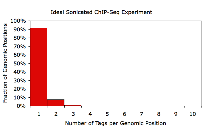
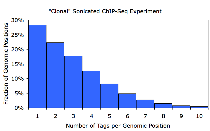
If an experiment looks like the bottom example, it's a good idea to redo the ChIP and re-prep the sample for sequencing.  This doesn't mean that useful information cannot still be gleamed from the sample, but it does mean that you are only getting a fraction of the information out that you are paying for.  As a rule of thumb, if your averageTagsPerPosition parameter in the tagInfo.txt file is less than 1.5, you are in good shape.  Again, this may not be an appropriate metric for RNA-Seq or enzymatically digested ChIP-Seq (i.e. MNase).

ChIP works by fragmenting crosslinked chromatin so that only pieces of DNA bound by a particular protein are purified.  As a result, and due to the requirements of DNA fragment length for efficient sequencing by next-generation sequencers, only DNA fragments of a particular size are used for ChIP-Seq.  This often involves cutting out a band of a specific size or range of sizes from a gel.  The specific size of fragments sequenced for a given experiment can be very important in extracting meaningful data and precisely determining the location of binding sites.

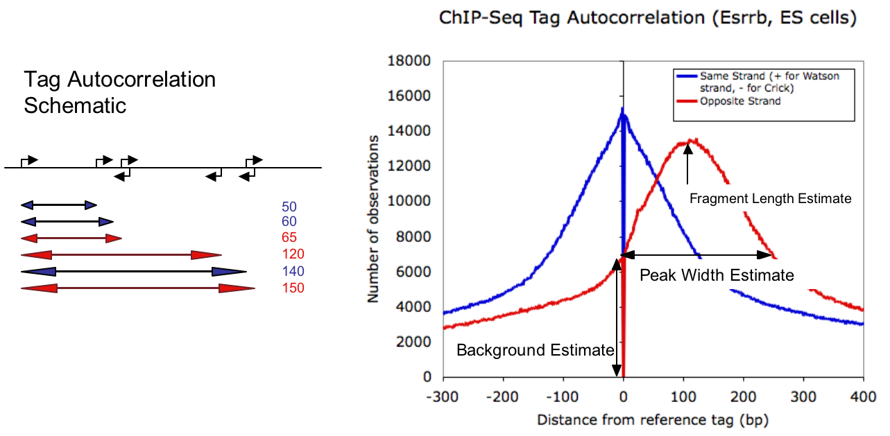
To estimate the length of fragments used for sequencing, we perform an autocorrelation analysis of tag positions.  This is done by calculating the distance from each tag to every other tag along the same chromosome and making a histogram of these distances, keeping track of which tags are found on the same strand or separate strands.  This is shown below:


The data to generate this plot is found in the tagAutocorrelation.txt file found in the tag directory.  Simply open it with EXCEL and make an x-y plot with the data.
NOTE: to change the parameters used to generate the tag autocorrelation, you can reanalyze the experiment using the autoCorrelateTags.pl tool.

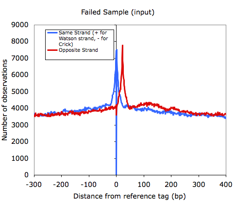
The tag autocorrelation is a nice piece of information for several reasons.  First, you can usually tell right off the bat if your experiment worked at all.  If there are enriched regions, then you should expect tags to be found in the vicinity of one another.  If the autocorrelation plot looks flat, or extremely spiky, that's a good sign something might have gone wrong with the experiment.

The other primary piece of information we extract from the autocorrelation is an estimate of the fragment length used for sequencing.  This estimate is derived from the maximum in autocorrelation signal in opposite strand tags found downstream of the reference tag (crest in the red signal above).  We can further estimate the relative range in fragment sizes by considering when the opposite strand distribution falls below its corresponding level at the reference tag (i.e. at zero).  Since tags found on opposite strands, facing away from each other cannot measure the same protein bound to the DNA, the level of opposite strand autocorrelation found at the origin provides an estimate of the background of the ChIP-Seq signal.  This value is then used to estimate the peak size (for transcription factors or other proteins that make contact at specific positions).  These values are stored in the tagInfo.txt file for automatic look up later.

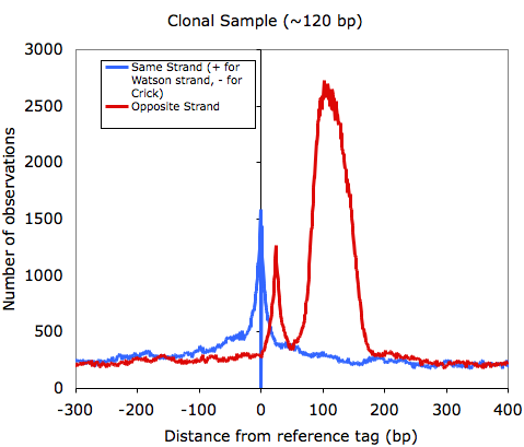
Other examples of tag auto correlations can be found below:


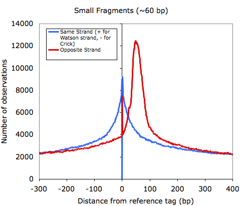
One thing I'll point out is that as the quality of samples decrease, the signal from tags mapping as palindromes increases.  For example, the
input (mock IP) control sample below shows a strong spike at 23 bp, which corresponds to the length of sequence used to map that sample.


If you sample is clonal (i.e. from the section above), it is common that you will see a high enrichment of opposite strand autocorrelation since you are essentially sequencing both ends of every fragment.


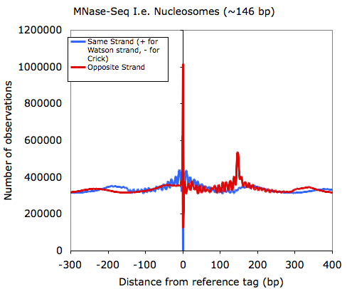
And for fun, because Chuck loves bioinformatics, you can do this with MNase-Seq data (which hints at how nucleosomes are organized)

HOMER checks for bias in your sequencing data by aligning every tag in its genomic context and calculating the nucleotide frequency at each position relative to the 5' end of the tag.  This can be useful for identifying bias in sequences produced by your experimental protocol, or sequencing issues, or problems with preferential sequencing of GC-rich vs. AT-rich regions.

For now, HOMER does NOT automatically analyzed sequence bias as part of the makeTagDirectory program (although this will change in the near future).  For now, this is handled by the program checkTagBias.pl.  The important parts of this program are written in C++ so it's fairly fast, even for large data sets.  To analyze your sequence bias for a tag directory, type the following:


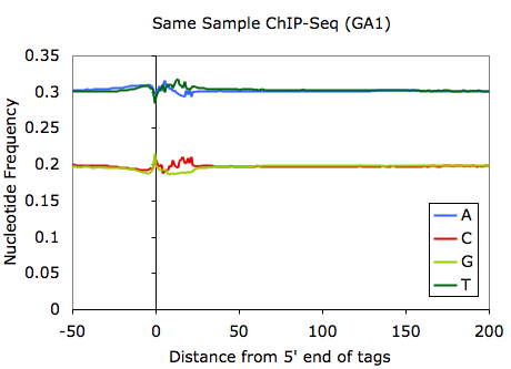
This requires that <genome> (in this case mm8) is loaded by homer (for more info click HERE).  This command will produce a file named tagFreq.txt in the tag directory.  Opening this file with EXCEL and graphing the first 5 columns will produce something like this:


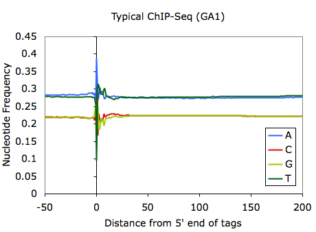
Although it may depend heavily on what is sequenced, most ChIP-Seq samples should look something like the above example.  It is very typical to have strong sequence preferences right at the 5' edge of the tag, where sequence preferences introduced by the ligation of sequencing adapters will enrich for fragments with specific sequences.  Variation within the first ~30 bp is normally indicative of bias from the base calling of the sequencer.

One observation worth noting is that sequencing performed on the Illumina GA2 (vs. GA1) tends to select for fragments that have higher overall GC-content.  For example (using the same sample):


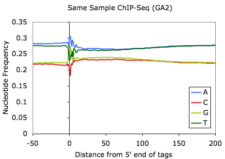
This unfortunately can bias where you might find peaks.  In extreme cases where experimental mishaps may have contributed, the GC-bias can be very extreme (see below):


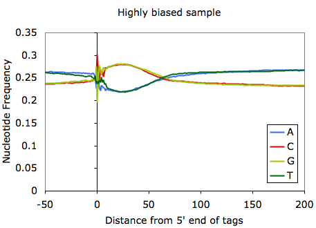
In this case you're basically screwed.  Since in most cases the fragments you pull down in the ChIP experiment are background anyway, you shouldn't see a major shift in GC-content in your ChIP-Seq fragments.  In the case above, you can also essentially approximate the length of the ChIP-Seq fragments (~55 bp according to the autocorrelation analysis).  Another way to check for GC-bias related problems is to check the files named tagGCcontent.txt and tagCpGcontent.txt in the tag directory after running checkTagBias.pl.  These files contain data describing the distribution of GC and CpG content for each fragment from sequencing.  Below is an example corresponding to the experiment shown above:


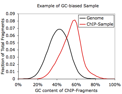
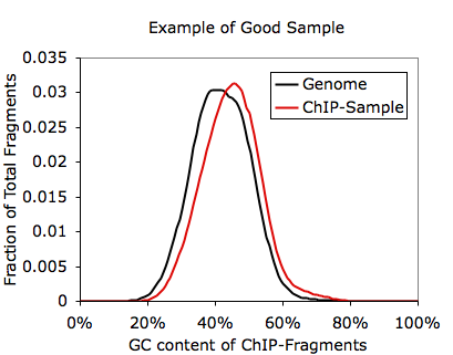
Obviously, if your sequencing looks like this, your peak finding will basically be blind to peaks in AT-rich regions of the genome.  In this case, the experiment needs to be repeated.

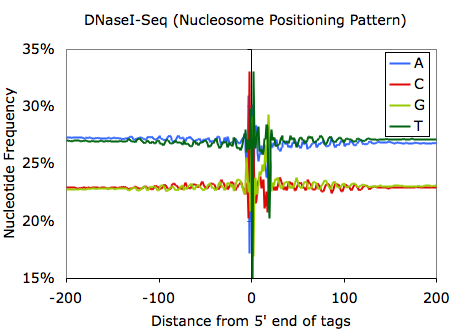
Sequencing bias can also be used for discovery; for example, the sequencing bias can reveal sequence preferences for restriction enzymes.  Examination of MNase- and DNaseI-digested DNA reveals the sequences that are preferentially cleaved by each enzyme:


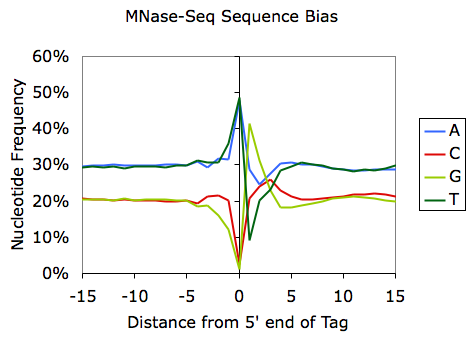
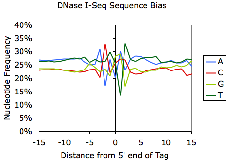
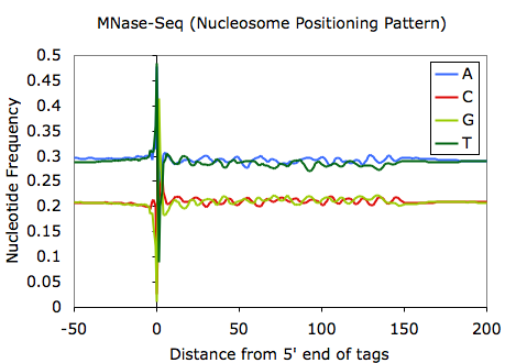
And if you ask Chuck, he'd tell you that you should zoom out on the MNase and DNase tag bias plots to reveal sequences that help position nucleosomes: