
HOMER
Software for motif discovery and ChIP-Seq analysis
ChIP-Seq Analysis: Annotating Peaks
Homer contains a useful, all-in-one program for performing peak
annotation called annotatePeaks.pl.
In
addition
to
associating
peaks
with
nearby genes, annotatePeaks.pl
can perform Gene
Ontology Analysis, associate peaks with gene expression data, calculate
ChIP-Seq Tag densities from different experiments, and find motif
occurrences in peaks. annotatePeaks.pl
can also be used to create histograms and heatmaps.!!! COMMON PROBLEM: If this program isn't working, make sure you save your peak files as "text (windows)" from EXCEL when on a Mac. Run the checkPeakFile.pl program to see if your file is the correct format, and use changeNewLine.pl if you didn't save your file in "text (windows)" format.
Basic usage:
annotatePeaks.pl
<peak
file>
<genome>
>
<output
file>
i.e. annotatePeaks.pl ERpeaks.txt hg18 > outputfile.txt
i.e. annotatePeaks.pl ERpeaks.txt hg18 > outputfile.txt
The first two argument, the <peak file> and <genome>, are required, and must be the first two arguments. Other optional command line arguments can be placed in any order after the first two. By default, annotatePeaks.pl prints the program output to stdout, which can be captured in a file by appending " > filename" to the command. With most uses of annotatePeaks.pl, an the output is a data table that is meant to be opened with EXCEL or similar program. An example of the output can been seen below:
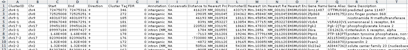
- Peak ID
- Chromosome
- Peak start position
- Peak end position
- Strand
- Peak Score
- FDR/Peak Focus Ratio
- Annotation (i.e. Exon, Intron, ...)
- Conservation
- Distance to nearest TSS
- Nearest TSS: Native ID of annotation file
- Nearest TSS: Entrez Gene ID
- Nearest TSS: Unigene ID
- Nearest TSS: RefSeq ID
- Nearest TSS: Ensembl ID
- Nearest TSS: Gene Symbol
- Nearest TSS: Gene Aliases
- Nearest TSS: Gene description
- Additional columns depend on options selected when running the program.
Adding Gene Expression Data
annotatePeaks.pl
can add gene-specific information to peaks based on each peak's nearest
annotated TSS. To add gene expression or other data types, first
create a gene data file (tab delimited text file) where the first
column contains gene identifiers, and the first row is a header
describing the contents of each column. In principle, the
contents of these columns doesn't mater. To add this information
to the annotation result, use the "-gene <gene data file>".
annotation.pl <peak file>
<genome> -gene <gene data file> > output.txt
For peaks that are near genes
with associated data in the "gene data file", this data will be
appended to the end of the row for each peak.
Gene Ontology Enrichment
annotatePeaks.pl
can automate the discovery of functionally enriched biological
annotations using the genes near ChIP-Seq peaks. Since this
analysis will produce several files, you must specify an output
directory with "-go <gene ontology output directory>".
Alternatively, you can run gene ontology directly on a list of gene IDs.
Calculating ChIP-Seq Tag Densities across different experiments
annotatePeaks.pl is useful
program for cross-referencing data from multiple experiments. In
order to count the number of tags from different ChIP-Seq experiments,
you must first create tag directories for
each of these experiments. Once created, tag counts from these
directories in the vicinity of your peaks can be added by specifying "-d <tag directory 1> <tag
directory 2> ...". You can specify as many tag
directories as you like. Tag totals for each directory will be
placed in new columns starting on column 18. For example:
HOMER automatically normalizes each directory by the total number of mapped tags such that each directory contains 10 million tags. This total can be changed by specifying "-norm <#>" or by specifying "-noadj", which will skip this normalization step.
The other important parameter when counting tags is to specify the size of the region you would like to count tags in with "-size <#>". For example, "-size 1000" will count tags in the 1kb region centered on each peak, while "-size 50" will count tags in the 50 bp region centered on the peak (default is 200). The number of tags is not normalized by the size of the region.
One last thing to keep in mind is that in order to fairly count tags, HOMER will automatically center tags based on their estimated ChIP-fragment lengths. This is can be overridden by specifying a fixed ChIP-fragment length using "-len <#>".
annotatePeaks.pl
pu1peaks.txt
mm8
-size
400
-d
Macrophage-PU.1/
Bcell-PU.1/ >
output.txt
output.txt, when opened in EXCEL, will look like this:
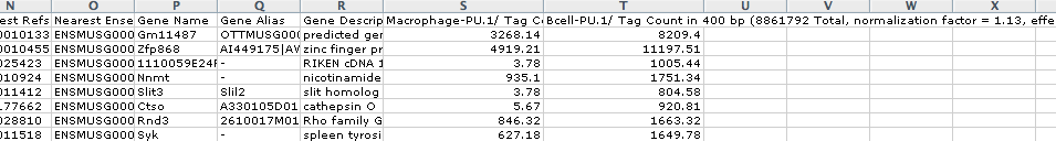
output.txt, when opened in EXCEL, will look like this:
HOMER automatically normalizes each directory by the total number of mapped tags such that each directory contains 10 million tags. This total can be changed by specifying "-norm <#>" or by specifying "-noadj", which will skip this normalization step.
The other important parameter when counting tags is to specify the size of the region you would like to count tags in with "-size <#>". For example, "-size 1000" will count tags in the 1kb region centered on each peak, while "-size 50" will count tags in the 50 bp region centered on the peak (default is 200). The number of tags is not normalized by the size of the region.
One last thing to keep in mind is that in order to fairly count tags, HOMER will automatically center tags based on their estimated ChIP-fragment lengths. This is can be overridden by specifying a fixed ChIP-fragment length using "-len <#>".
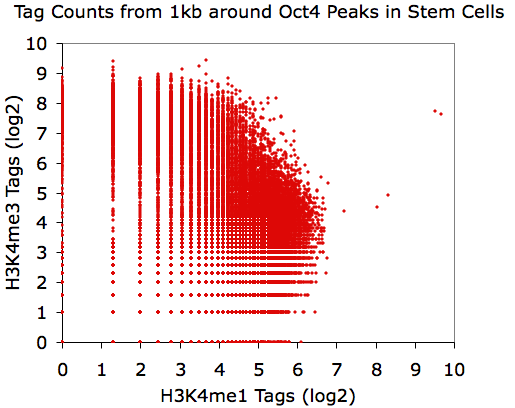
Making Scatter Plots
X-Y scatter plots are a great way
to present information, and by counting tag densities from different
tag directories, you can visualize the relative levels of different
ChIP-Seq experiments. Because of the large range of values, it
can be difficult to appreciate the relationship between data sets
without log transforming the data (or sqrt to stay Poisson
friendly). Also, due to the digital nature of tag counting, it
can be hard to properly assess the data from a X-Y scatter plot since
may of the data points will have the same values and overlap. To
assist with these issues, you can specify "-log" or "-sqrt" to transform the data.
These functions will actually report "log(value+1+rand)" and
"sqrt(value+rand)", respectively, where rand is a random "fraction of a
tag" that adds jitter to your
data so that data points with low tag counts will not have exactly the
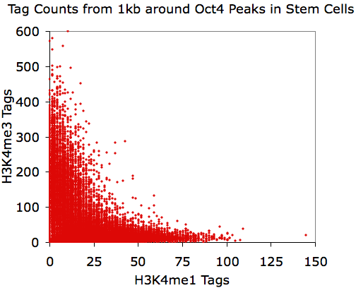
same value. For example, lets look at the distribution of H3K4me1 and
H3K4me3 near Oct4 peaks in mouse embryonic stem cells:
annotatePeaks.pl Oct4.peaks.txt mm8 -size 1000 -d H3K4me1-ChIP-Seq/ H3K4me3-ChIP-Seq/ > output.txt
Now using the "-log" option:
annotatePeaks.pl Oct4.peaks.txt mm8 -size 1000 -log -d H3K4me1-ChIP-Seq/ H3K4me3-ChIP-Seq/ > output.txt
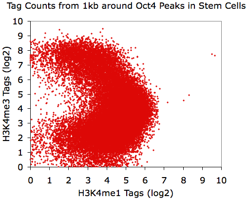
Believe it or not, all of these X-Y plots show the same data.
Interesting, eh?
annotatePeaks.pl Oct4.peaks.txt mm8 -size 1000 -d H3K4me1-ChIP-Seq/ H3K4me3-ChIP-Seq/ > output.txt
Opening output.txt with EXCEL
and plotting the last two columns:
Using EXCEL to take the log(base 2) of the data:
Using EXCEL to take the log(base 2) of the data:
annotatePeaks.pl Oct4.peaks.txt mm8 -size 1000 -log -d H3K4me1-ChIP-Seq/ H3K4me3-ChIP-Seq/ > output.txt
Finding instances of motifs near peaks
Figuring out which peaks have
instances of motifs found with
findMotifsGenome.pl is very easy. Simply use "-m <motif file1> <motif file
2>..." with annotatePeaks.pl.
(Motif
files
can
be
concatenated
into
a single file for ease of
use) This will search for each of these motifs near each peak in
your peak file. Use "-size
<#>" to specify the size of the region around the peak
center you wish to search. Found instance of each motif will be
reported in additional columns of the output file. For example:
annotatePeaks.pl pu1peaks.txt mm8 -size 200 -m pu1.motif cebp.motif > output.txt
annotatePeaks.pl pu1peaks.txt mm8 -size 200 -m pu1.motif cebp.motif > output.txt
Opening output.txt with EXCEL:
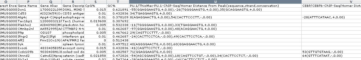
Each instance of the motif is
specified in the following format (separated by commas):
Distance from
Peak Center(Sequence
Matching Motif,Strand,Average
Conservation)
The average conservation will not
be reported unless you specify "-cons",
and
that
will
only
work
if
conservation information has been configured
(not available for all genomes). I wouldn't worry about
this. Also, when finding motifs, the average CpG/GC content will
automatically be reported since it has to extract peak sequences from
the genome anyway.
There are a bunch of motif specific options such as "-norevopp" (only search + strand relative to peak strand for motifs), "-nmotifs" (just report the total number of motifs per peak), "-rmrevopp <#>" (tries to avoid double counting reverse opposites within # bps).
There are a bunch of motif specific options such as "-norevopp" (only search + strand relative to peak strand for motifs), "-nmotifs" (just report the total number of motifs per peak), "-rmrevopp <#>" (tries to avoid double counting reverse opposites within # bps).
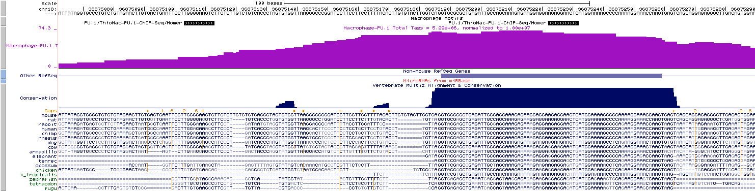
Visualizing Motif positions in the UCSC Genome Browser
This feature may seem slightly
out of place, but since annotatePeaks.pl is the workhorse of HOMER, you
can add "-mbed <filename>"
in
conjunction
with
"-m <motif file
1> [motif file 2] ..." to produce a BED file describing motif
positions near peaks that can be loaded as a custom track in the UCSC
genome browser. In the example below, you would load motif.bed as a custom track:
annotatePeaks.pl pu1peaks.txt mm8
-size 200 -m pu1.motif cebp.motif -mbed motif.bed >
output.txt
Finding the distance to other sets of Peaks
In order to find the nearest peak
from another set of peaks, use "-p
<peak file 1> [peak file 2] ...". This will add
columns to the output spreadsheet that will specify the nearest peak ID
and the distance to that peak. If all you want is the distance
(so you can sort this column), add the option "-pdist" to the command.
Otherwise, if you prefer to count the number of peaks in the peak file
found within the indicated regions (i.e. with "-size <#>"), add "-pcount".
Command line options for annotatePeaks.pl
Usage: annotatePeaks.pl <peak file | tss> <genome version> [additional options...]Available Genomes (required argument): (name,org,directory,default promoter set)
Peak vs. TSS mode:
If the first argument is "tss" (i.e. annotatePeaks.pl tss mouse ...) then a TSS centric
analysis will be carried out. Tag counts and motifs will be found relative to the TSS.
(no position file needed)
NOTE: The default TSS peak size is 4000 bp, i.e. +/- 2kb (change with -size option)
-list <gene id list> (subset of genes to perform analysis [unigene, gene id, accession,
probe, etc.], default = all promoters)
-TSS <promoter set> (promoter definitions, default=genome default)
-cTSS <promoter position file i.e. peak file> (should be -2000 to +2000 centered on TSS,refseqIDs)
Available Promoter Sets (use with -TSS): (name,org,directory,genome,masked genome)
Primary Annotation Options:
-m <motif file 1> [motif file 2] ... (list of motifs to find in peaks)
-mscore (reports the highest log-odds score within the peak)
-nmotifs (reports the number of motifs per peak)
-fm <motif file 1> [motif file 2] (list of motifs to filter from above)
-rmrevopp <#> (do not double count reverse opposite motif occurrences, # bp window to look for them)
-d <tag directory 1> [tag directory 2] ... (list of experiment directories to show
tag counts for) NOTE: -dfile <file> where file is a list of directories in first column
-p <peak file> [peak file 2] ... (to find nearest peaks)
-pdist to report only distance (-pdist2 gives directional distance)
-pcount to report number of peaks within region
-gene <data file> ... (Adds additional data to result based on the closest gene.
This is useful for adding gene expression data. The file must have a header,
and the first column must be a GeneID, Accession number, etc. If the peak
cannot be mapped to data in the file then the entry will be left empty.
-go <output directory> (perform GO analysis using genes near peaks)
-matrix <filename> (outputs a motif co-occurrence matrix)
-mbed <filename> (Output motif positions to a BED file to load at UCSC | -mpeak <filename>)
Annotation vs. Histogram mode:
-hist <bin size in bp> (i.e 1, 2, 5, 10, 20, 50, 100 etc.)
The -hist option can be used to generate histograms of position dependent features relative
to the center of peaks. This is primarily meant to be used with -d and -m options to map
distribution of motifs and ChIP-Seq tags. For ChIP-Seq peaks for a Transcription factor
you might want to use the -center option (below) to center peaks on the known motif
NOTE: tss Mode is OK
Histogram Mode specific Options:
-nuc (calculated mononucleotide frequencies at each position,
Will report by default if extracting sequence for other purposes like motifs)
-di (calculated dinucleotide frequencies at each position)
-histNorm <#> (normalize the total tag count for each region to 1, where <#> is the
minimum tag total per region - use to avoid tag spikes from low coverage
-ghist - outputs profiles for each gene, for peak shape clustering - only uses first directory
-rm <#> (remove occurrences of same motif that occur within # bp)
Peak Centering: (other options are ignored)
-center <motif file> (This will re-center peaks on the specified motif, or remove peak
if there is no motif in the peak. ONLY recentering will be performed, and all other
options will be ignored. This will output a new peak file that can then be reanalyzed
to reveal fine-grain structure in peaks (It is advised to use -size < 200) with this
to keep peaks from moving too far (-mirror flips the position)
-multi (returns genomic positions of all sites instead of just the closest)
Advanced Options:
-log (output tag counts as randomized log2 values - for scatter plots)
-sqrt (output tag counts as randomized sqrt values - for scatter plots)
-size # (Peak size[from center of peak], default=inferred from peak file)
-size #,# (i.e. -size -10,50 count tags from -10 bp to +50 bp from center)
-size "given" (count tags etc. using the actual regions - for variable length regions)
-local # (size in bp to count tags as a local background (10-100x peak size recommended)
-len # (Fragment length, default=150)
-pc # (maximum number of tags to count per bp, default=0 [no maximum])
-cons (Retrieve conservation information for peaks/sites)
-CpG (Calculate CpG/GC content)
-ratio (process tag values as ratios - i.e. chip-seq, or mCpG/CpG)
-norevopp (do not search for motifs on the opposite strand [works with -center too])
-noadj (do not adjust the tag counts based on total tags sequenced)
-norm # (normalize tags to this tag count, default=1e7, 0=average tag count in all directories)
-pdist (only report distance to nearest peak using -p, not peak name)
-noann (skip annotation step)
Back to ChIP-Seq Analysis

Can't figure something out? Questions, comments, concerns, or other feedback:
cbenner@ucsd.edu